Fine-tuning foundation models with biological priors

2026-08-15

We use modern AI methods where they are useful. For us, they are modelling tools rather than a product category. We also think some of the best-funded work in biological AI has a fundamental gap which is being ignored. It is a limit imposed by the data used to train the models.

The problem is familiar in language models. Most people can now recognise recurrent ChatGPT or Claude constructions such as “it is not just X, but Y” or “that is not the hard part; the hard part is…”. These patterns are learned from statistical structure in the training data or reinforcement. Biological foundation models inherit the same constraint, although the artefacts are much harder to recognise.

A model trained on ClinVar classifications, gnomAD frequencies, sequence embeddings, protein-effect predictions, and expression measurements can learn extremely useful relationships between those quantities. It cannot infer information that was never represented. A pathogenic ClinVar label does not encode the probability that two rare alleles occur together in trans under a recessive inheritance model. An allele frequency does not say whether that genotype explains a phenotype. An absent variant call does not say whether the site was confidently resolved or simply beyond the effective sensitivity of the assay.

A model trained on end-point labels can become very good at reproducing those labels while remaining poor at simulating the biology that generated them. That becomes a serious limitation when the model is used to design an antibody, select neoantigens for a personalised cancer vaccine, predict the effect of a novel genomic alteration, or optimise a molecule against a protein target. These tasks depend on the biological states and transitions that produce the observed outcome. Simplified observational categories capture only one sixth of the evidence space described by the underlying Bayesian causal probabilities.

More parameters do not restore that missing information. More GPUs do not restore it. Fine-tuning for another ten epochs does not restore it. The information has to exist in the representation supplied to the model.

This is where we are focused. We model the biological event itself. That means assigning probabilities to admissible events under population, inheritance, genotype, phenotype, and measurement assumptions. It requires handling complex realities such as a dominant genetic allele, a homozygous genotype, a compound heterozygous pair in trans, and an unresolved structural event are different objects with different probabilities.

Consider an autosomal recessive disease. Two rare variants in the same gene may each have a ClinVar classification, an allele frequency, and a predicted or known protein effect. The causal event is the genotype containing the relevant pair in trans. We calculate the probability of that event under the relevant population and inheritance model before patient-specific evidence is added.

Biology has always required this kind of probabilistic description. Perrin’s experiments on Brownian motion showed that apparently random molecular motion could be described quantitatively. Hardy and Weinberg formalised expected allele frequencies under inheritance, and Fisher and Wright extended population genetics to selection, drift, mutation, and migration. Modern computation changes the scale at which these processes can be modelled, but the requirement is unchanged: the data must represent the process that generates the observation.

Sutton’s Bitter Lesson gives the corresponding argument for machine learning. General methods have repeatedly improved as data and computation increased. That principle works only when the data preserve the information the model needs to learn. In genetics, collapsing inheritance, measurement state, and causal configuration into downstream annotations creates an information ceiling before training has even begun.

We have been building the missing quant layer. It includes inheritance-conditioned event probabilities, population priors, genotype configurations, phenotype context, and explicit measurement states for resolved and unresolved evidence. These quantities can enter Bayesian models directly or become structured inputs for training and fine-tuning foundation models.

A simple desktop example

Our biological models become technically dense quickly, and the detailed methods contain sensitive intellectual property. A smaller text-classification problem lets us show the same fine-tuning process with familiar data and a model that you can reproduce on a laptop.

We follow biotechnology news closely. Company formation, acquisitions, clinical results, and scientific developments are useful signals, so we want incoming articles classified according to categories that help us decide what to read.

Training a language model from the beginning would make little sense for this task. Luckily, there are many public models available already. distilbert-base-uncased is one which is already pretrained to represent English text. It has learned statistical structure from a large general-language corpus, so words, sentences, and their context already have useful internal representations. What it has not learned is our classification task. It does not know that we want an article assigned to a specific niche like “Bayesian statistical models”. In our simple example we stick to more general labels. The news articles are labelled as World, Sports, Business, or Sci/Tech.

Hugging Face provides the pretrained DistilBERT model and its tokenizer through the Transformers library. It also provides the labelled AG News dataset through the Datasets library. PyTorch handles the numerical training itself, including the forward pass, loss calculation, gradients, and parameter updates.

For this blog post, we fine-tuned the model on 1,000 labelled AG News articles, with 500 articles for validation and an untouched 500-article test set. Training used one epoch, batch size 8, a maximum sequence length of 128 tokens, and AdamW with a learning rate of 5e-5.

A new four-class classification layer is attached to the pretrained DistilBERT representation. Before fine-tuning, that layer has not learned how the four labels relate to the text, so performance sits close to the 0.25 chance level expected from four balanced classes. It achieved 0.238 accuracy and 0.139 macro F1. After one CPU training epoch, held-out accuracy reached 0.888 and macro F1 reached 0.886.

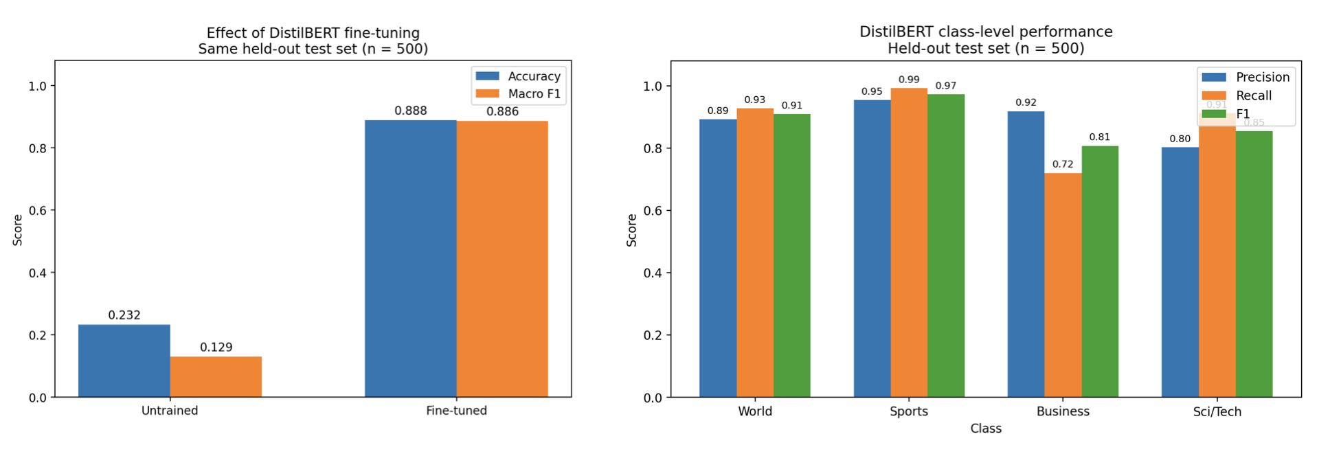
The class-level results show where the model still makes mistakes. Sports reached 0.99 recall, while Business recall was 0.72. Several Business articles were classified as Sci/Tech, which is relevant for biotechnology monitoring because acquisitions often contain financial and scientific language in the same article.

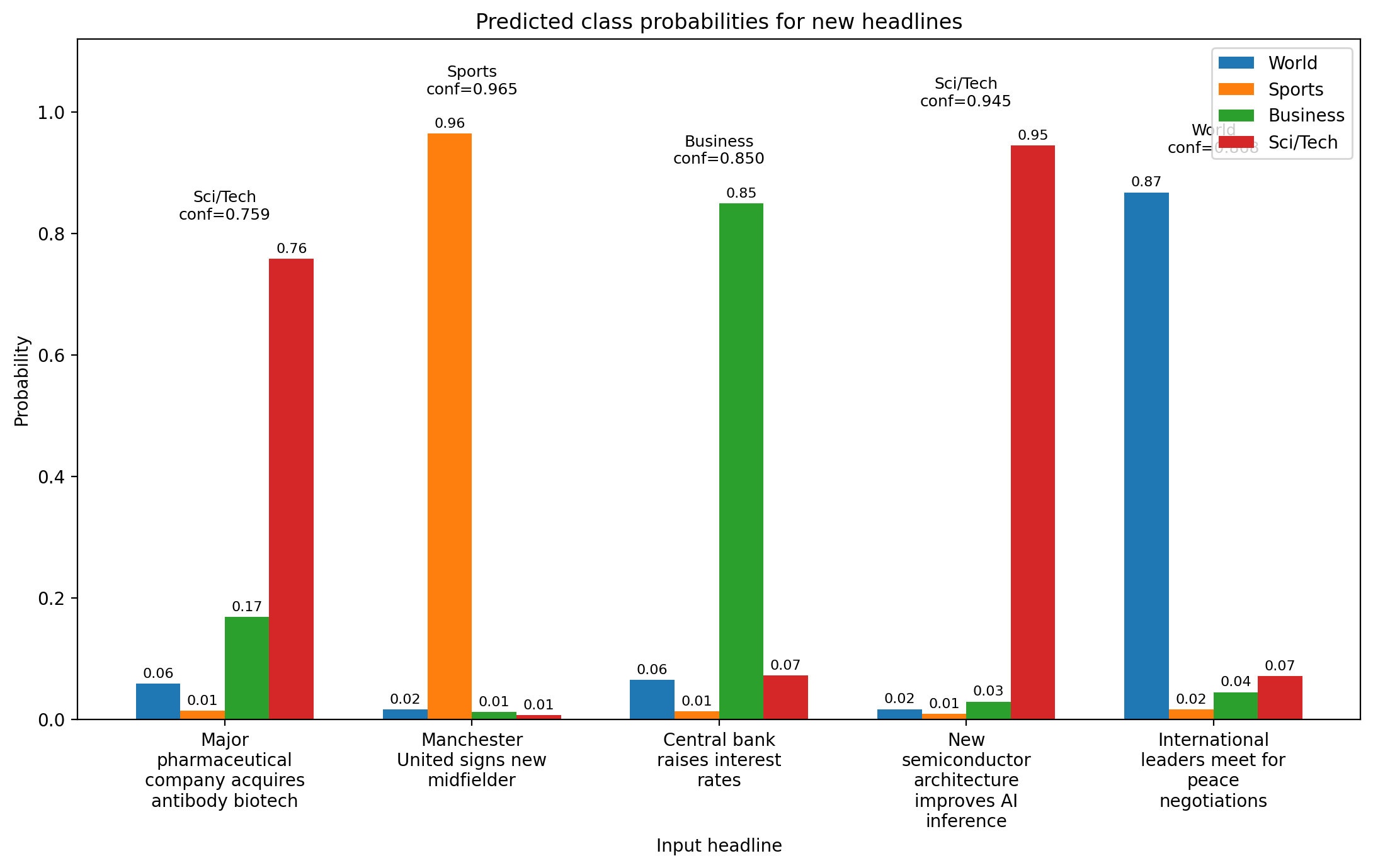
The saved model can then classify previously unseen headlines. For Major pharmaceutical company acquires antibody biotech, the output was:

Sci/Tech   0.759
Business   0.168
World      0.059
Sports     0.014

Keeping the full probability vector is useful for monitoring. Articles can be ranked by score, and different categories can use different thresholds. Mixed scientific and commercial content can retain that ambiguity rather than being reduced immediately to one hard label.

This experiment ran on an older laptop. The model is deliberately small, but the underlying training process is the same one used for larger models:

pretrained model
→ task-specific representation
→ forward pass
→ loss
→ backpropagation
→ parameter update
→ validation
→ held-out evaluation
→ inference

From article labels to genetic events

A genetic model receives a very different representation. For a rare-disease model, an input may contain population frequency, genotype configuration, mode of inheritance, ancestry, phenotype context, predicted molecular consequence, protein structure, gene expression, functional evidence, and assay resolution. Each field describes a different part of the process. Graph representation is also sometimes more relevant for biological interactions.

A simplified dominant event might look like:

population frequency         2.1e-5
inheritance model            dominant
proband genotype             heterozygous
parental observation         absent
molecular consequence        missense
protein domain               annotated
structural effect            predicted
gene expression              measured
gene-disease evidence        curated
assay state                  resolved

A recessive event is different because the causal unit is generally the genotype configuration rather than either allele in isolation. For two candidate alleles (i) and (j), one possible hypothesis is:

The frequency of each allele contributes to the probability of that genotype under the relevant population model. Mode of inheritance changes the event definition. Phase changes whether the pair is admissible. Phenotype context changes which events belong in the model.

This information can be represented before patient-specific evidence is added:

population and inheritance model
→ admissible genetic events
→ event-level priors
→ patient-specific observations
→ model update
→ posterior probabilities

The event space includes variants that were not observed. A plausible splice variant may fall in a poorly covered region. A second recessive allele may remain unresolved. A structural event may fall outside the sensitivity of the assay.

That distinction is encoded through a measurement model. If (G_i) is the underlying genetic state and (M_i) describes the assay and calling process, the observed evidence (X_i) depends on both:

An alternate call, a confidently resolved reference state, and an unresolved site are therefore different observations. They should have different effects on the probability assigned to a genetic hypothesis.

What the model is asked to predict

The target needs the same precision as the input. A model of molecular effect might estimate whether a substitution changes protein stability. An expression model might estimate the effect of a variant on RNA abundance. A somatic model might estimate driver probability. A genetic model might estimate the probability that an observed event will later receive causal support under a specified phenotype and inheritance model.

These are different quantities. Training labels and validation data should reflect the quantity being estimated. Sutton’s Bitter Lesson, mentioned earlier, is worth returning to here: scalable learning works best when the model discovers the structure itself, rather than inheriting our simplified view of the problem.

This is why solving the statistical and computational problems that make biological complexity modelable is so useful. It brings real-world evidence into the model that simplified labels leave out. A ClinVar label can describe accumulated evidence about a variant. It does not encode the probabilities of molecular consequence in a single cell or system. Two alleles with strong individual annotations may still have a very different joint probability once allele frequencies, phase, ancestry, and inheritance are considered.

Our work focuses on making those quantities explicit and modelable.

Sequence context can enter through an embedding from a genomic foundation model. Protein sequence or structure can enter through another representation. Population frequency can remain numerical. Genotype configuration, inheritance, phase, and assay state can remain structured variables. These components can then be combined for statistical inference or model training.

Probability in the two examples

The news classifier returns softmax scores. A value of 0.90 means that the classifier assigned 90% of its output mass to one of its learned categories. It is useful for ranking and classification, but it is not automatically a calibrated 90% probability that an external biological statement is true.

For genetic events, we define the probability explicitly. The prior describes the distribution over admissible events before the current patient observation is incorporated. Patient-specific evidence then changes that distribution.

This separation also prevents the same evidence from entering the calculation twice. Population information used to construct an event prior remains identifiable. Patient sequence evidence remains identifiable. Molecular or functional evidence can be introduced at the appropriate stage.

A complete hypothesis space can also retain a null model, unresolved alternatives, and events outside the current model scope. Posterior probability is therefore not forced into the small set of variants visible in one VCF, for example.

Scaling to HPC

The DistilBERT example for this blog post ran on CPU because the model and dataset were small. Larger transformer models spend much of their training time performing dense matrix operations. PyTorch uses CUDA to execute those operations efficiently on NVIDIA GPUs.

An illustrative HPC allocation might be:

1 compute node
2 × NVIDIA A100 80 GB
32 CPU cores
256 GB RAM
local NVMe scratch
8 DataLoader workers per GPU
PyTorch
CUDA
Slurm
bfloat16 mixed precision
checkpoint after each epoch

The GPUs execute the model forward pass, gradient calculation, and parameter updates. CPU cores handle operations such as genomic file parsing, decompression, feature construction, and preparation of upcoming batches. Eight DataLoader workers per GPU might be a reasonable starting point for this allocation, although the correct value depends on profiling.

The 80 GB of memory on each A100 constrains model size, batch size, and context length. The 256 GB of system RAM provides working memory for decoded genomic data and preprocessing. Local NVMe scratch can reduce repeated access to a slower shared filesystem.

Mixed precision can reduce GPU memory use and increase throughput. bfloat16 is particularly useful on hardware that supports it because it retains a wider exponent range than float16.

GPU utilisation then shows whether the input pipeline is keeping pace. If the GPU repeatedly becomes idle, preprocessing or storage may be the bottleneck. Increasing DataLoader workers, staging data locally, or precomputing expensive representations may improve throughput. Adding CPU cores after the GPU is already continuously supplied with data provides little benefit.

Multiple GPUs add gradient synchronisation. PyTorch DistributedDataParallel can divide the workload across devices, but the throughput gain must justify the communication cost.

Validation with genetic data: a fascinating headache

Multi-omic datasets contain dependencies that a random variant-level split can easily miss. Several variants may come from one patient. Several patients may come from one family. The same recurrent variant may appear in many individuals. Several examples may come from the same gene, ancestry group, sequencing site, or assay.

The split therefore depends on the scientific claim. A rare-disease model may require family-level separation. A gene-effect model may require gene-level holdout. Population generalisation may require testing in a distinct ancestry cohort.

External validation can deliberately change one source of variation. A model can be trained in one ancestry and tested in another. It can be trained on data from one sequencing laboratory and evaluated in another. Assay platforms and independent clinical cohorts can be tested separately.

Calibration, class imbalance, missing evidence, subgroup performance, batch effects, and distribution shift can then be measured directly rather than inferred from aggregate accuracy.

Reproducible runtime

The final part is the engineering discipline that turns research into something another organisation can depend on. The algorithms and databases are an exciting part of the work. Releasing them to a biotechnology company, pharmaceutical team, or hospital requires another layer of engineering. A result has to be reproducible months later, on another machine, by another team, with the exact model, evidence, and software environment that produced it.

We therefore version the entire computational lineage. The Git commit identifies the source code. The foundation-model checkpoint identifies the starting parameters. The dataset release identifies the training observations. The dependency lock records the Python packages. PyTorch and CUDA versions identify the numerical runtime. Training checkpoints preserve model and optimiser state.

For HPC deployment, the validated environment can be packaged as an Apptainer or OCI container. The image digest identifies the exact executable environment. The final model receives an immutable version, and the associated data release carries its own identifier. A company or hospital should be able to determine exactly which model checkpoint, container image, evidence release, and code commit produced a result.

Our biological models require the same care with the science itself. Event definitions, inheritance-conditioned priors, measurement states, reference assumptions, and unresolved evidence all belong to the model lineage. A change to any of them creates a new version that can be tested, compared, and released deliberately.

This infrastructure takes a large amount of work, and most users will never see it. They should not have to. What matters is that when a result is used in a real pipeline, every component behind it can be traced, reproduced, and defended.

Foundation models will continue to improve, but domain-specific performance will still depend on how they are adapted. Fine-tuning remains one of the clearest ways to bring specialised biological data, priors, and objectives into those models.