
2026-09-19
Most people now encounter language models through systems such as ChatGPT. You supply text, and the model produces a response. The underlying process is less visible: how does a neural network learn from text in the first place, and what happens mathematically when it generates the next word or character?
Some of our time is devoted to ML/AI methods. This is usually focused on genomic sequences and protein structures. We enjoy understanding these systems from first principles, including the mathematics behind how they learn. For this blog we built a small language model entirely in R to examine that process directly. It uses a vanilla recurrent neural network (RNN) trained from randomly initialised parameters on an ordinary laptop CPU. It allows anyone to follow the learning process and judge the results without specialist biological knowledge.
There are no pretrained weights, Python dependencies, GPU operations or deep-learning frameworks performing automatic differentiation. Python is now the standard language for AI development, but it is not a requirement. We work extensively in R, so we built this language model entirely from first principles in base R, rather than adapting a pre-existing implementation or relying on a deep-learning framework. The forward pass, loss calculation, gradients and parameter updates are implemented using base R matrix operations.
The objective is to understand the complete learning algorithm rather than reproduce the capabilities of a modern language model. The model learns one task: given the characters it has already encountered, predict the next character.
Our implementation follows the mathematics of Andrej Karpathy’s 2015 minimal character-level RNN which he discussed here and here. We have separated the model from data preparation and experiment control, and added validation, reproducible checkpoints, tests and visual monitoring so that we can examine what happens during training.
Where this fits in AI history
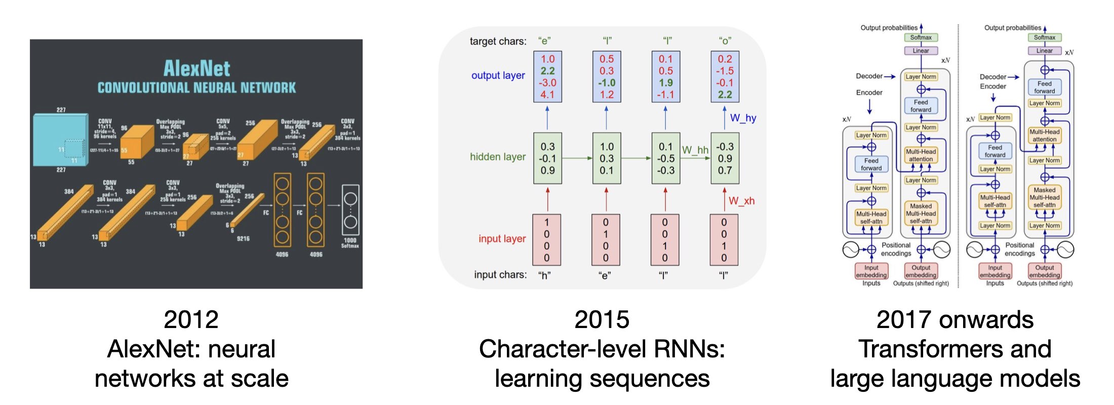
Neural networks were already being used to learn patterns in data long before modern generative AI. An important reference point is AlexNet, published in 2012. It used a deep convolutional neural network with approximately 60 million parameters to classify images into 1,000 categories. Its training dataset contained approximately 1.2 million labelled images, and training took several days on two GPUs.
AlexNet demonstrated what could be achieved by combining neural network architectures with substantial datasets and computational resources. It was an image classifier, however, rather than a language model. Recognising an object in an image is a different prediction problem from learning how a sequence of text continues.
Recurrent neural networks address sequential data by maintaining a hidden state that changes as each new input arrives. Earlier recurrent architectures were developed before AlexNet, and Long short-term memory (LSTMs) subsequently introduced mechanisms for retaining and discarding information across longer sequences. Karpathy’s minimal RNN is a compact example of this family: it learns directly from characters and generates text by repeatedly predicting what comes next.
The next major architectural development for language modelling was the Transformer, introduced in the 2017 paper Attention Is All You Need. Rather than requiring all information about preceding text to pass through one recurrent hidden state, Transformer layers use attention to combine information from different positions in a sequence. This architecture supports a different way of representing context and is well suited to large-scale parallel computation during training.
GPT-2, released in 2019, used a decoder-only Transformer with up to approximately 1.5 billion parameters, trained on a large collection of web text. Modern frontier language models operate at much greater computational and data scale than our small RNN, and their complete training procedures can include additional stages beyond next-token pretraining.
The important distinction is that the underlying learning task remains recognisable even when the architecture changes. A model receives a numerical representation of text, calculates predictions, compares those predictions with the observed continuation and adjusts its parameters using the resulting gradients.
Our experiment isolates that process in a network small enough to implement and inspect completely.
From text to a prediction problem
We use the Tiny Shakespeare dataset, containing 40,000 lines, consisting of 1,115,394 characters of dialogue and other text. The first step is to identify its unique characters and assign each one an integer index. Spaces, punctuation, capitalisation and newline characters are retained.
$ wc data/tiny_shakespeare.txt
40000  202651 1115394 data/tiny_shakespeare.txt

$ head data/tiny_shakespeare.txt
First Citizen:
Before we proceed any further, hear me speak.

All:
Speak, speak.

First Citizen:
You are all resolved rather to die than to famish?
For our experiment, the vocabulary contains 65 unique characters. Every character is represented by a one-hot vector with 65 positions: the position corresponding to that character is set to one and all other positions are zero. Unlike a pretrained tokenizer, this encoding does not already contain information about words or their meanings.
The training objective is created directly from the original text. Consider the short sequence The king:
| Current character | Actual next character |
|---|---|
T |
h |
h |
e |
e |
space |
| space | k |
k |
i |
i |
n |
n |
g |
The network receives T and predicts the next character. The correct answer is h, because that is what appears next in the training text. It then receives the actual h, predicts the next character again and continues through the sequence.
No manually assigned language labels are required. The original text supplies both the inputs and the correct targets at every position.
This also establishes a limitation of the task: the network is learning the statistical structure of character sequences. It is not being directly trained to establish whether a sentence is factually correct or whether its meaning is useful.
How the recurrent network works
A conventional feedforward network processes an input without necessarily retaining information from the preceding inputs. An RNN introduces a hidden state that is updated as successive characters arrive.
For each character, our network combines its current one-hot input with the hidden state produced at the previous step:
\[h_t=\tanh(W_{xh}x_t+W_{hh}h_{t-1}+b_h).\]Here, (x_t) represents the current character and (h_{t-1}) represents the preceding hidden state. The two weight matrices and bias determine how the current input and previous context contribute to the new hidden state.
The model then converts that state into an output score for every character in its vocabulary:
\[p_t=\operatorname{softmax}(W_{hy}h_t+b_y).\]The softmax operation converts the scores into a probability distribution that sums to one. If the input is T, the model might assign a high probability to h, with smaller probabilities assigned to other possible next characters.
The hidden state is what makes this more than a simple character-frequency table. The same character can lead to different predictions depending on the characters encountered before it. For example, an h following T occurs in a different context from an h appearing at the end of a word.
Our implementation uses 100 hidden neurons. With a vocabulary of 65 characters, the input, recurrent and output weight matrices, together with their biases, contain 23,165 trainable parameters.
The same parameters are reused at every character position. The model does not construct a different neural network for every step; its hidden state changes while its learned matrices remain shared across the sequence.
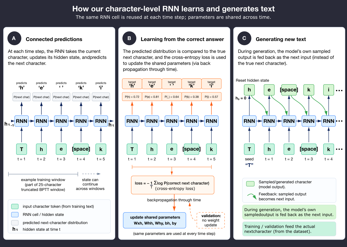
Figure 1. A character-level RNN processes successive input characters through shared recurrent parameters. Each hidden state contributes to the prediction of the next character and passes information to the next time step. During generation, predicted characters are fed back into the network instead of the actual continuation from the dataset.
How the network learns
At the beginning of training, the model’s weights are randomly initialised. Its predictions are initially close to uninformative. For a vocabulary of 65 equally probable characters, the expected next-character cross-entropy loss is:
\[L_{\mathrm{uniform}}=\log(65)\approx4.174\]nats per character.
Training compares the probability assigned to each correct next character with the character that actually appears in the text. If the model assigns a probability of 0.8 to the correct next character, its loss for that position is:
\[L_t=-\log(0.8)\approx0.223.\]Assigning a lower probability to the correct character produces a larger loss. The objective is to reduce the average loss across the training sequence by adjusting the learned parameters.
Those adjustments require gradients: numerical quantities describing how changes to each parameter affect the loss. In an RNN, an earlier hidden state can influence several later predictions, so the gradients must account for the connections between successive time steps. This is calculated using backpropagation through time.
Our implementation processes training sequences in windows of 25 characters. Gradients are propagated backward through the current window, while the resulting hidden state can be carried into the following window. This is truncated backpropagation through time: the model can retain information across windows during the forward pass, but each parameter update only backpropagates through the current window.
We calculate these gradients explicitly in R and use AdaGrad to update the parameters. AdaGrad maintains an accumulated squared-gradient value for each parameter and uses it to adjust the size of subsequent updates. We also clip individual gradient values to limit unusually large updates.
No external library calculates the derivatives or performs the optimisation. The R implementation exposes the operations that are normally handled by a deep-learning framework.
What validation measures
A falling training loss tells us that the network is improving its predictions on the text used to update its parameters. It does not establish that those improvements apply to text the network has not trained on.
We therefore divide the corpus into a training portion and a contiguous held-out validation portion. Training updates the parameters using only the training text. Validation evaluates the same next-character prediction task on the held-out text without updating any parameters.
For example, if the validation text contains The king, the model predicts the next character after T and measures the probability it assigned to the actual h. It then receives the actual h and predicts the following e, continuing through the passage.
The validation loss is the average negative log probability assigned to those actual next characters. A lower value means the model assigned higher probabilities, on average, to the observed continuation.
This is different from asking the model to generate a passage and judging whether it sounds convincing. Validation always supplies the actual preceding characters, so we can calculate its prediction error against known targets.
Our current experiment evaluates a fixed 2,000-character portion of the held-out validation text at regular checkpoints. This makes repeated measurements comparable and keeps evaluation inexpensive, but it is not a complete measurement across the entire held-out corpus.
Generating new text
Text generation uses the same trained parameters but changes how the model receives its next input.
During training and validation, the actual next character from the dataset is supplied at each step. During generation, we start with a seed character and allow the network to select its own continuation.
Suppose we start with T. The model calculates a probability distribution for the next character and samples one possibility, perhaps h. It then receives that generated h, updates its hidden state and samples another character. The process continues until the requested number of characters has been produced.
Each generated character becomes the input for the following step. There is no correct continuation supplied by the dataset, and no parameter update takes place during generation.
Our runner periodically generates a new passage using the model parameters learned up to that training iteration. The generation hidden state is reset for each passage, but the learned parameters are retained. A sample generated after 15,000 training updates therefore comes from a differently trained model than a sample generated after 5,000 updates. It is not an extension of the earlier passage.
This separation between learning and generation is important. During learning, the dataset defines the correct continuation. During generation, the model must continue from its own previous outputs, so an improbable or unusual sampled character can influence everything that follows.
What we observed on a laptop CPU
We trained the network on Tiny Shakespeare using 100 hidden neurons, a sequence length of 25 and AdaGrad with an initial learning rate of 0.1.
Our first experiment completed 5,000 parameter updates in approximately one minute. Validation loss fell from approximately 4.174 to 2.556 nats per character. Generated samples began to contain recognisable words, spaces, punctuation and fragments of dialogue, although they were not consistently grammatical.
A subsequent 50,000-update experiment produced a more interesting learning curve. Its lowest measured validation loss was approximately 2.246 at 41,000 updates, while the final validation loss was approximately 3.314. Training loss remained much lower and changed relatively smoothly, whereas validation loss increased sharply around 30,000 updates, recovered near 41,000 and deteriorated again.
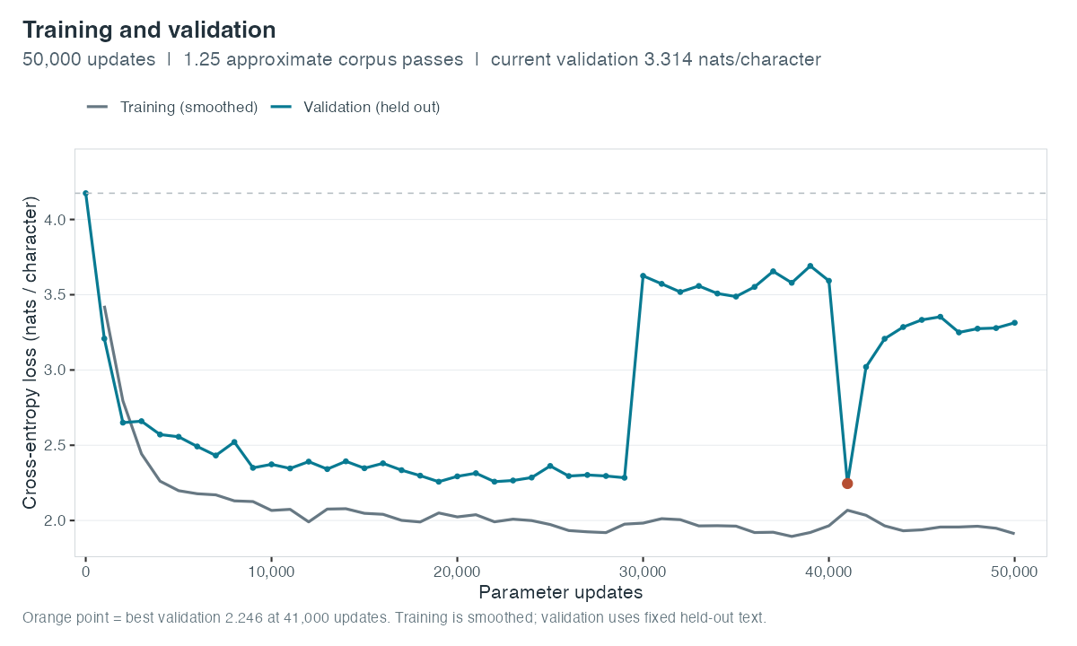
Figure 2. Training and validation loss during 50,000 updates. Training loss is exponentially smoothed; validation loss is measured on the same fixed held-out passage. The best recorded validation checkpoint occurs at 41,000 updates rather than at the end of training.
The declining training loss shows that the network continued improving its predictions on recent training sequences. The validation curve shows that these improvements did not consistently transfer to the measured held-out passage.
We cannot determine the cause of those abrupt changes from this graph alone. The experiment reads the training corpus sequentially, uses a relatively small recurrent network and evaluates only a fixed portion of the validation corpus. The effects of training order, parameter updates and validation-passage selection would need to be tested separately before attributing the changes to one mechanism.
The example also demonstrates why the final model is not necessarily the most useful checkpoint. We preserve the parameters associated with the lowest measured validation loss so that they can be compared with the parameters obtained at the end of training.
There is another important distinction in scale. At a sequence length of 25, 50,000 parameter updates process approximately 1.25 million character positions, or about 1.25 passes through our training split. That is a small amount of training by the standards of modern language models, even though it is sufficient to observe recognisable learning behaviour.
Training longer, adjusting the learning rate and evaluating a larger held-out sample may improve our measurements and generated text. They do not remove the architectural limitations of a small vanilla RNN, particularly its difficulty retaining useful information across long passages.
What this teaches us about larger language models
Our network contains only 23,165 learned parameters and operates on individual characters. GPT-2, by comparison, used up to approximately 1.5 billion parameters and was trained on a much larger text corpus using a Transformer architecture.
The difference is not only parameter count. Our RNN compresses preceding context into a recurrent hidden state and processes characters sequentially. A Transformer uses attention and multiple learned transformations to represent relationships between positions in a context window. Larger models also use different token representations, training procedures and computational infrastructure.
Nevertheless, several essential operations remain familiar: text is converted into numerical inputs, learned parameters produce predictions, a loss function measures disagreement with observed data, gradients determine parameter updates, and the trained model generates a continuation from its previous context.
Implementing the small network in R makes those operations directly observable. We can inspect the weight matrices, calculate the gradients ourselves, check them against numerical derivatives, observe the training and validation curves and restore the parameters from an earlier checkpoint.
The exercise does not reproduce a modern frontier language model. It establishes, using an entire implementation that fits in a small codebase, how a neural network can learn a language-modelling objective from data and turn its learned parameters into new text.
The complete source code, experiment runner, tests and monitoring tools are available in the accompanying project.
References
Krizhevsky A, Sutskever I, Hinton GE. (2012). ImageNet Classification with Deep Convolutional Neural Networks.
Karpathy A. (2015). The Unreasonable Effectiveness of Recurrent Neural Networks and Minimal character-level RNN implementation.
Vaswani A, Shazeer N, Parmar N, et al. (2017). Attention Is All You Need.
Radford A, Wu J, Child R, et al. (2019). Language Models are Unsupervised Multitask Learners.


