Building a character-level Transformer in R

2026-09-21

We sometimes develop AI models for biological data, including genomic sequences and protein structures. To make the underlying algorithms easier to understand on the blog, we are rebuilding them from first principles in R, using ordinary text so readers can follow the mathematics and learning process without specialist biological knowledge.

Building on our previous work with recurrent neural networks (RNNs), we now reproduce a small, GPT-like Transformer from first principles in R. Unlike RNNs, which process text sequentially through a recurrent hidden state¹, the Transformer uses causal self-attention to process positions within a context window in parallel, while preventing each position from accessing future characters.

In practice this means the model can directly compare each character with all others in its context, without carrying a hidden state forward. This avoids the long-range dependency issues of RNNs and makes training much faster. In fact, Vaswani et al. report that Transformers train up to an order of magnitude faster than comparable recurrent models. Figure 1 shows the core architecture of our minimal character-level Transformer: character+position embeddings → one causal self-attention block (with a feed-forward sublayer) → output scores for the next character.

The code is available here https://github.com/switzerlandomics/src-min_char_transformer_r.

We use the Tiny Shakespeare dataset, containing 40,000 lines, consisting of 1,115,394 characters of dialogue and other text. The first line of text reads “First Citizen: Before we proceed…”, which you will recognise in some of the figures below as the prompt: F i r s ….

$ wc data/tiny_shakespeare.txt
40000  202651 1115394 data/tiny_shakespeare.txt

$ head data/tiny_shakespeare.txt
First Citizen:
Before we proceed any further, hear me speak.

All:
Speak, speak.

First Citizen:
You are all resolved rather to die than to famish?

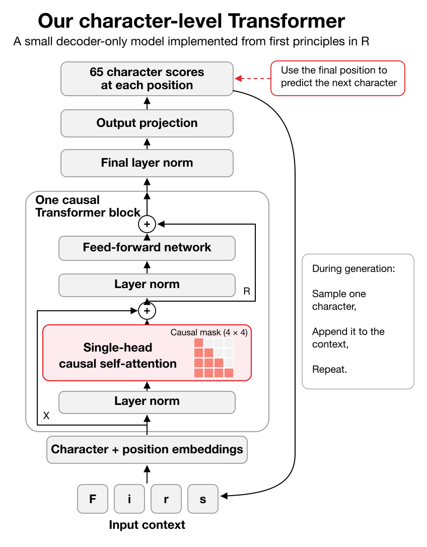
Figure 1. The implemented Transformer model. Input characters (“F i r s”) are first converted to learned character and position embeddings, summed to form the input matrix \(X\). We then apply one “Transformer block” (pre‑layer‑norm, single-head self-attention plus a feed-forward network, each with residual connections). The output vector at the final position is projected to produce unnormalized logit scores over the 65-character vocabulary, which are passed through softmax to give the next-character probabilities.

RNNs versus Transformers

Traditional sequence models like RNNs process tokens sequentially. Each new input updates a hidden state that carries information forward. This sequential dependence makes RNNs inherently slow to train (since they cannot parallelize over positions) and prone to forgetting information over long distances due to vanishing gradients. For example, determining that “bank” refers to a river bank might require an RNN to propagate information across many intermediate words.

By contrast, a Transformer sees the whole context at once. It replaces recurrence with self-attention: at each layer, every position computes queries, keys and values to attend to all other positions simultaneously. Positional embeddings are added so the model knows each token’s order. In practice this means:

• Parallel processing: All input positions are processed in parallel, greatly reducing training time.
• Global context: Each token’s representation can incorporate information from any other token in the window, not just the last hidden state.
• Positional encoding: The model learns fixed or learned positional embeddings so that it still “knows” which character is first, second, etc..

Figure 2 illustrates this contrast. In the RNN (left), characters are fed one by one and each step carries a hidden state forward. In the Transformer (right), all characters are embedded and then interact through self-attention in a single block.

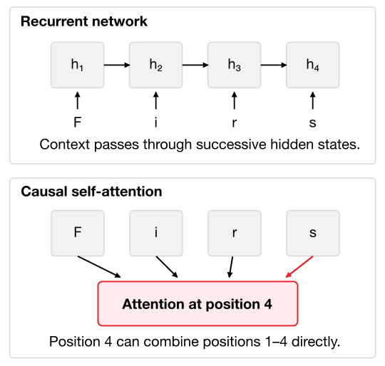
Figure 2. In an RNN (left), characters are processed sequentially with a hidden state passed from one step to the next. The Transformer (right) processes all input positions in one go using self-attention (no recurrent hidden state). The Transformer’s positional embeddings (⊕) preserve order, and each position attends to all others simultaneously.

Transformer model details

Our implementation follows the decoder-only Transformer style (like GPT) with one attention block. Given a sequence of \(n\) input characters encoded as indices, we look up both character embeddings and learned positional embeddings (each of dimension \(d\)), and sum them to form an input matrix \(X\in\mathbb{R}^{n\times d}\). This matrix is then layer-normalised before entering the self-attention sublayer (we use the “pre-LN” variant).

Within the self-attention sublayer, we compute queries (\(Q\)), keys (\(K\)), and values (\(V\)) as linear projections of the normalised input \(H=\operatorname{LN}_1(X)\):

where \(W_Q,W_K,W_V\in\mathbb{R}^{d\times d}\) are learned weight matrices. The scaled dot-product attention is then

Here, \(M\) is the causal mask: it prevents each position from attending to characters that come after it.

This applies softmax row-wise to the masked query–key scores, producing attention weights between 0 and 1 that sum to 1 for each query. In other words, each query position \(i\) computes a weighted sum of the value vectors from its current and earlier positions. The weights are determined by the compatibility (scaled dot product) between that query and each permitted key.

Because our model has a single attention head, we use only one set of these projections. After attention, we add its output to the original input through a residual connection. We then apply layer normalisation before a position-wise feed-forward network,

which consists of two linear transformations with a ReLU activation between them. A second residual connection completes the Transformer block, followed by a final layer normalisation.

Finally, we multiply the resulting representations by an output weight matrix \(W_{\mathrm{out}}\in\mathbb{R}^{d\times65}\) and add a bias to obtain logits for all 65 characters at every input position. During generation, we use the logits at the final input position and apply softmax to obtain a probability distribution from which to sample the next character.

In summary, our forward pass is:

• Embed characters + positions → \(X\).
• Compute one masked self-attention output matrix \(A\) (above).
• Feed \(A\) through the feed-forward sublayer to get \(Y\).
• Output logits \(z = Y_n W_o + b_o\) for the final position \(n\).
• Probabilities \(p = \text{softmax}(z)\) for the next character.

Each step involves simple linear algebra and nonlinearity, making the math straightforward yet expressive. Figure 3 (next section) shows how we apply the mask to ensure the model is autoregressive during generation.

Causal masking for autoregression

To use the Transformer for language modeling, we must enforce causality: when predicting each character, the model should not see future characters in the sequence. We implement this with a causal mask on the attention. Concretely, in the matrix \((QK^T)/\sqrt{d}\) we add large negative values (effectively \(-\infty\)) wherever \(j>i\), so that the softmax assigns zero weight to those positions. In practice this means each query position \(i\) can only attend to itself and earlier key positions.

Figure 3 illustrates this: cells above the diagonal (future positions) are shaded off-white and receive no weight. The allowed (unmasked) cells use a color scale (red) proportional to the actual attention weight. For decoding, a token cannot attend to tokens not yet generated. Thus, the self-attention module in the decoder is causally masked.

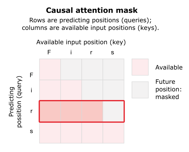
Figure 3. Causal masking in self-attention. White cells are masked (future positions) and have zero weight; only the allowed cells (below the diagonal) are colored according to attention weight. Each row is a query position and shows which previous keys it can attend to. This ensures the model cannot “see” future characters when generating text.

One prediction step: the math

Putting it all together for a single input window, the Transformer computes next-character probabilities as follows:

1. Embedding: Form matrix \(X\in\mathbb{R}^{n\times d}\) by summing character and position embeddings for the \(n\) input characters.
2. Compute Q,K,V: As above, \(Q=XW_Q\), \(K=XW_K\), \(V=XW_V\).
3. Dot-Product: Compute scaled dot-products \(S = QK^T/\sqrt{d}\) (an \(n\times n\) matrix).
4. Apply mask: Set \(S_{i,j}=-\infty\) for all \(j>i\) (future tokens).
5. Softmax: Apply \(\text{softmax}\) to each row of \(S\) to obtain attention weights.
6. Weighted sum: \(A = \text{softmax}(S) \, V\), so that \(A_{i} = \sum_j (\text{softmax}(S)_{i,j})\,V_j\). Row \(i\) of \(A\) is the attended output for query \(i\).
7. Feed-forward: For each row \(A_i\), apply \(F(A_i) = W_2\mathrm{ReLU}(W_1A_i + b_1) + b_2\) and add the residual connection.
8. Output projection: Take the last output vector \(F(A_n)\) and compute logits \(z = F(A_n)W_o + b_o\).
9. Softmax: Finally \(p = \text{softmax}(z)\) gives the probability distribution for the next character.

Figure 4 schematically illustrates this process for our four-character prompt “Firs” (characterized by vectors on the left). The core operation is attention: each query vector is dotted with key vectors, scaled by \(\sqrt{d}\), and normalized to form the weight matrix. As Glass Box Medicine explains, after softmax we have “attention weights” that sum to 1 for each row, and we use those to combine the value vectors. The resulting output at position 4 (for “s”) feeds into the final softmax. (Layer norms and residuals are omitted in the diagram for clarity.)

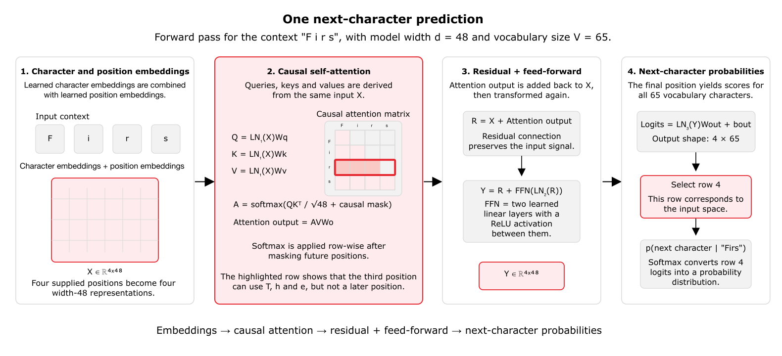
Figure 4. The forward-pass computations for one Transformer prediction step on input “F i r s”. The input characters are embedded and added to position embeddings. We compute queries/keys/values (Q,K,V) and form the scaled dot-product matrix \(QK^T/\sqrt{d}\). After masking future positions, we apply softmax row-wise to obtain attention weights, which weight-sum the rows of \(V\). The attention outputs are then passed through a feed-forward layer. The final output vector at position 4 is projected to 65 logits and softmaxed. (Residual connections and layer norms are applied at each sub-layer, as in Figure 1.)

Training and evaluation

We train this model on the Tiny Shakespeare dataset (a corpus of Shakespeare plays) using maximum likelihood. At each step, the model is given a sequence of \(n=128\) characters (we accumulated overlapping windows, training on all positions). The true next character for each position provides a cross-entropy loss; we sum the losses over the \(n\) positions and backpropagate to update all parameters. We use the Adam optimizer with default settings.

Figure 5 plots the training loss and held-out validation loss (in nats per character) over 300,000 updates. The uniform baseline (log loss of a uniform model over 65 symbols, about 4.1744 nats/char) is shown near the top of the plot, and a bigram baseline (using single-character frequencies given the previous char) is also indicated. Even early in training the Transformer far outperforms these naive baselines. Both curves decrease as the model learns; the lowest validation loss recorded was about 1.7472 nats/char at 295,000 updates, which is where we saved the final checkpoint. (At that point, our model was selected for text generation in our blog example.)

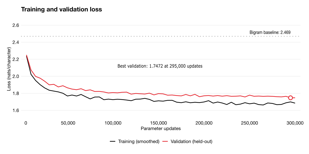
Figure 5. Training and validation loss (in nats/character) over 300k updates for the Transformer. Training loss is exponentially smoothed for clarity. The uniform baseline (no knowledge of text) has loss ≈4.1744; the bigram baseline is about 2.4692. The model quickly improves, reaching ~1.75 nats/char on validation by 295k updates. The red dot marks the best validation checkpoint (1.7472 nats at 295,000 updates), which we use for generation.

Our implementation reproduces the expected behavior: given the same prompt Firs, it predicts and samples the same continuation as recorded in our “generation comparison” (see our experiments folder). The code and training logs are available in the repository for full transparency.

Learned attention weights

Finally, we visualize the actual attention weights learned by the model for the prompt Firs. Figure 6 shows the 4×4 attention matrix from the best checkpoint. Each row corresponds to a query position (1 through 4 for “F”, “i”, “r”, “s”, and each column corresponds to a key position. Masked (future) positions are white. The colored cells show the weight (importance) assigned to each permitted key by that query. For example, row 4 shows how the model at “s” distributes attention over {F,i,r,s}. We annotate this figure with a colorbar for clarity.

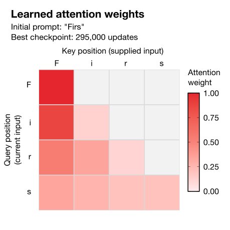
Figure 6. Actual attention weights from the best-validation checkpoint, for the input “F i r s”. Each row is one query position, each column one key position. Off-white cells were masked (future positions) and have weight 0. The color intensity indicates how much attention that query paid to each allowed key. The model’s attention is automatically normalized (each row sums to 1). These patterns show how, for each position, the model is combining its context. (For example, later positions tend to assign more weight to recent characters.) Importantly, every position has direct access to all earlier positions, a property known to help learning long-range dependencies.

Have we reached AGI yet?

In this blog post we have implemented a minimal Transformer language model in R, from the ground up. We covered the intuition and math behind self-attention, causally masked generation, and multi-layer feed-forward networks. The figures illustrate how the Transformer fundamentally differs from an RNN, how it computes its predictions, and how well it trains on real data. Importantly, all our results come from the same learned model (no hand-tuning of the figures), demonstrating the approach’s correctness.

Like our previous RNN example, this exercise highlights that modern deep learning architectures can be understood and built using simple code and math. Our Transformer uses only 1 head and 1 layer, but it still effectively captures sequence patterns in the Shakespeare text. The same principles scale to larger models and datasets. In future work we will extend this to even longer contexts and explore the Transformer’s applications in omics sequence data.

End results

As with the previous RNN blog post, we are not too concerned with producing eloquent poetry. We are mostly focused on accurate math and model design - once that is in place we can simply scale on larger hardware.

The initial run at a validation around 4 shows basically random nonsense:

Update 0 - validation 4.18 - prompt “Firs”

xg.BFPFbzvfMYbBwA  

tZrQqRZy3jmrhtngmq;!  

aWaSpLHIf'eauW,kDNOd,P;  
DLUVCjasqLZGPwpoIMwrg3&  
lThgLsyqhFQ-SSuw!Kfj$ml  
pAw.zdesCxn'q?&&?$T*

After a short time it starts to have a recognisable structure:

Update 250,000 - validation 1.77 - prompt “Firs”

First stand in till if royar douceving
Clinif;
You must! cousin and figher
To way that lend
And loves not a thee
This be burgice is pabarandy, do brich nigh;
Net me town.

NORTHUMB:
Go

update 260,000 - validation 1.76 - prompt “Firs”

First utsern sunfried rests 
and to galinght that 
dear's cope heaving in the utbuar in 
must at and smethere batted?

CORIOLANUS:
Host gaitie, splaint is she pevers
Inf, sirving there wa

Update 295,000 - validation 1.74 - prompt “Firs”

e
Maring weld sound, a
That look; our pressay
cause cold ostandont: sot, so both unfame,
Unbuit me whost to be bood eson.
Comful
To and my gal my greath fooble, that you,
She no b

The generated text remains imperfect, but the lower validation loss and increasingly recognisable structure show that our single-block Transformer learns from text on a laptop CPU. Built entirely from first principles in R, it demonstrates a core mechanism of the 2017 Transformer architecture. Our next project will extend this work to a deeper GPT-2-style model.

The training data and code are provided in the src-min_char_transformer_r repository on GitHub.

References

Vaswani A, Shazeer N, Parmar N, et al. (2017). Attention Is All You Need, https://arxiv.org/abs/1706.03762 . Advances in Neural Information Processing Systems, 30.