Building a GPT-2-style language model from scratch in R

2026-09-25

We sometimes develop AI methods for genomic sequences and protein structures. For this series, we rebuild the underlying models from first principles in R using ordinary text, so the mathematics can be examined without specialist biological knowledge.

A generative pre-trained transformer (GPT) is a decoder-only Transformer trained to predict the next token from the tokens that precede it. The Transformer introduced self-attention, allowing positions within a sequence to interact directly while training can be parallelised across positions [Vaswani et al., 2017]. GPT used a decoder-only stack with causal attention, in which each position can use earlier tokens but not future ones [Radford et al., 2018].

Here we reproduce the main computational structure of GPT-2 in R. Our model uses byte tokens, learns token and position embeddings, multi-head causal self-attention, independently parameterised Transformer blocks, GELU feed-forward layers and tied input/output embeddings. The complete forward pass, backward pass, cross-entropy loss and Adam updates are implemented directly with R matrices and arrays, without a deep-learning framework or automatic differentiation.

In our open-source implementation min-GPT2 from scratch no external packages were used. We train or evaluate the model using basic R. ggplot2 and svglite were used only to produce figures on this page. The parameters begin as random numbers and are learned from Tiny Shakespeare on a laptop CPU.

The code is available here https://github.com/switzerlandomics/src-min_gpt2_r.

We use the Tiny Shakespeare dataset, containing 40,000 lines, consisting of 1,115,394 characters of dialogue and other text. The first line of text reads “First Citizen: Before we proceed…”, which you will recognise in some of the figures below as the prompt: F i r s ….

$ wc data/tiny_shakespeare.txt
40000  202651 1115394 data/tiny_shakespeare.txt

$ head data/tiny_shakespeare.txt
First Citizen:
Before we proceed any further, hear me speak.

Where GPT-2 fits

GPT-1 combined generative pre-training with supervised adaptation to individual language tasks [Radford et al., 2018]. The model first learned by predicting text, then used the resulting parameters as the starting point for supervised task-specific training.

GPT-2 showed that a substantially larger decoder-only Transformer trained on web text could perform several tasks directly from textual context, without task-specific parameter updates [Radford et al., 2019]. Its largest version contained approximately 1.5 billion parameters. The important change was not the invention of autoregressive language modelling, but the range of behaviour produced by scaling a single next-token prediction objective.

GPT-2 also attracted attention outside machine-learning research. OpenAI initially released smaller models while delaying the complete 1.5-billion-parameter checkpoint, then released the full model later in 2019 [OpenAI, 2019a; OpenAI, 2019b]. The staged release made general-purpose language generation part of a broader discussion about increasingly capable models.

GPT-3 extended the same scaling direction to 175 billion parameters and demonstrated substantially stronger in-context learning [Brown et al., 2020]. ChatGPT, released in 2022, subsequently made conversational language models directly accessible to a broad public audience [OpenAI, 2022]. GPT-2 therefore occupies an important intermediate position between the introduction of generative Transformer pre-training and the later public adoption of large language models.

Our model for this blog post is many orders of magnitude smaller. The largest experiment described here contains 369,504 trainable parameters and uses a context of 96 byte tokens. Its purpose is to expose the main computations in a form that can be inspected completely.

From a Transformer to GPT-2

Our previous project implemented one causal self-attention head in one Transformer block. A GPT-2-style model extends this structure with multiple heads, independently parameterised blocks, pre-layer normalisation, GELU feed-forward layers and a final layer normalisation.

For an input representation \(X\), one block computes

followed by

Here, \(\operatorname{LN}\) is layer normalisation, \(\operatorname{MHA}\) is multi-head attention, \(\operatorname{FFN}\) is the feed-forward network, \(H\) is the intermediate representation after attention, and \(Y\) is the block output.

The residual additions preserve a direct path through the block, while attention and the feed-forward network learn transformations of the current representation. The output \(Y\) becomes the input to the next independently parameterised block.

Our largest experiment uses three blocks, four attention heads and an embedding dimension of 96. Each head therefore operates on 24 features.

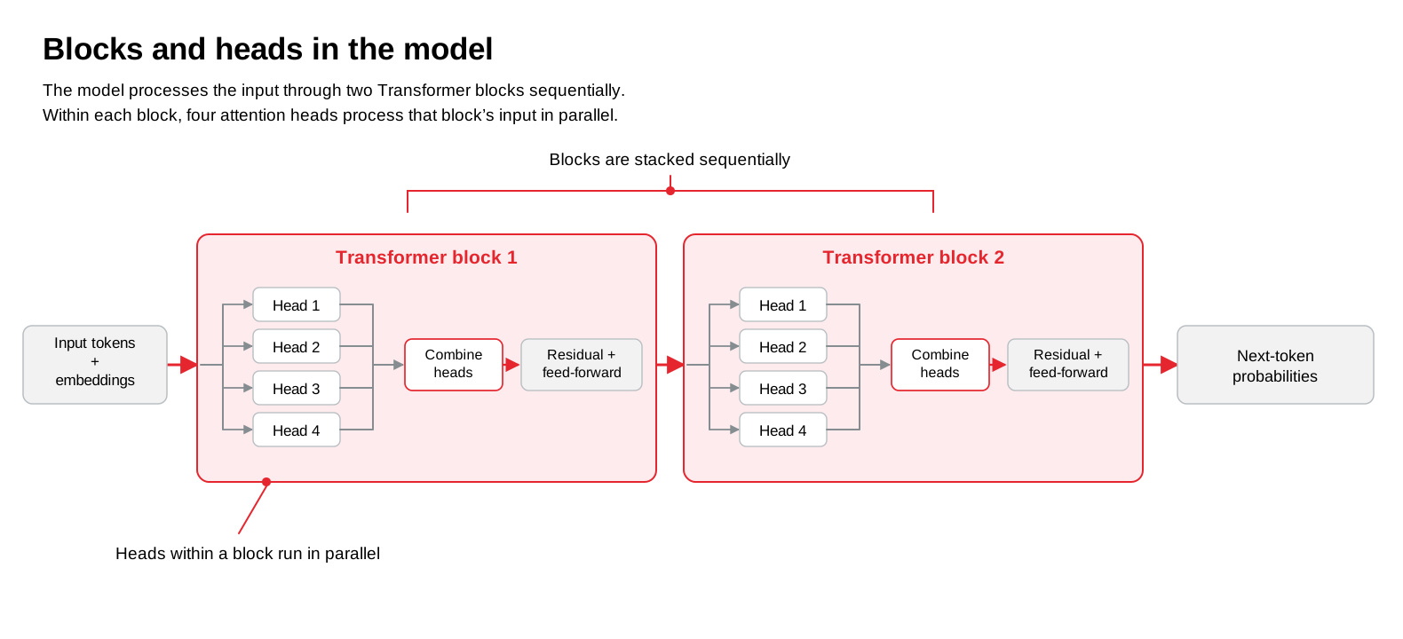
Figure 1. Stacked blocks and multiple attention heads. Our largest model uses three independently parameterised Transformer blocks. Within each block, the 96-dimensional representation is divided across four 24-dimensional attention heads, recombined by an output projection and passed through the residual and feed-forward paths.

Tokens and context

A language model operates on numerical token IDs rather than text directly. GPT-2 used byte-level byte-pair encoding (BPE), which builds a vocabulary of frequently occurring byte sequences and can represent arbitrary text [Radford et al., 2019]. Its released tokenizer contains 50,257 token IDs.

Our tokenizer deliberately stops one step earlier. Each UTF-8 byte maps directly to one of 256 token IDs, using the byte value plus one because R indexes from one. The ASCII text you are, therefore contains eight tokens. No vocabulary is learned from the corpus, and no token already represents a complete word or common subword.

This choice separates the Transformer from the tokenisation algorithm. It makes the mapping between the original file and the model input exact, while retaining a fixed vocabulary capable of representing arbitrary UTF-8 byte sequences. It is simpler than GPT-2’s BPE and usually requires more tokens to represent the same text.

The corpus is read as raw bytes and divided contiguously into 80% training, 10% validation and 10% test data. A training window pairs every input token with the token that follows it. For example,

input:   First Ci
target:  irst Cit

Every position therefore supplies a next-token training example.

Each token ID selects a row from a learned token-embedding matrix \(E\), and each position \(t\) selects a learned position embedding \(P_t\). For token \(x_t\) at position \(t\),

The resulting vectors \(X_t\) form the initial sequence representation passed to the first Transformer block.

Multi-head causal attention

Multi-head causal attention allows several attention operations to act on different feature subspaces of the same sequence. A single linear projection produces query (\(Q\)), key (\(K\)) and value (\(V\)) representations, whose feature dimension is then divided across the heads.

For head \(i\),

where \(Q_i\), \(K_i\) and \(V_i\) are the query, key and value matrices for that head, \(d_h\) is its feature dimension, and \(M\) is the causal mask. Entries above the diagonal are set to \(-\infty\) before softmax, so their attention weights become zero and a position cannot use future tokens.

The \(h\) head outputs are concatenated and projected back to the embedding dimension,

where \(\operatorname{MHA}\) denotes multi-head attention, \(X\) is the input sequence representation and \(W_O\) is the learned output-projection matrix.

The four heads in our largest model therefore calculate four separate attention matrices for the same sequence. Their outputs are combined before the residual connection returns the result to the common 96-dimensional representation.

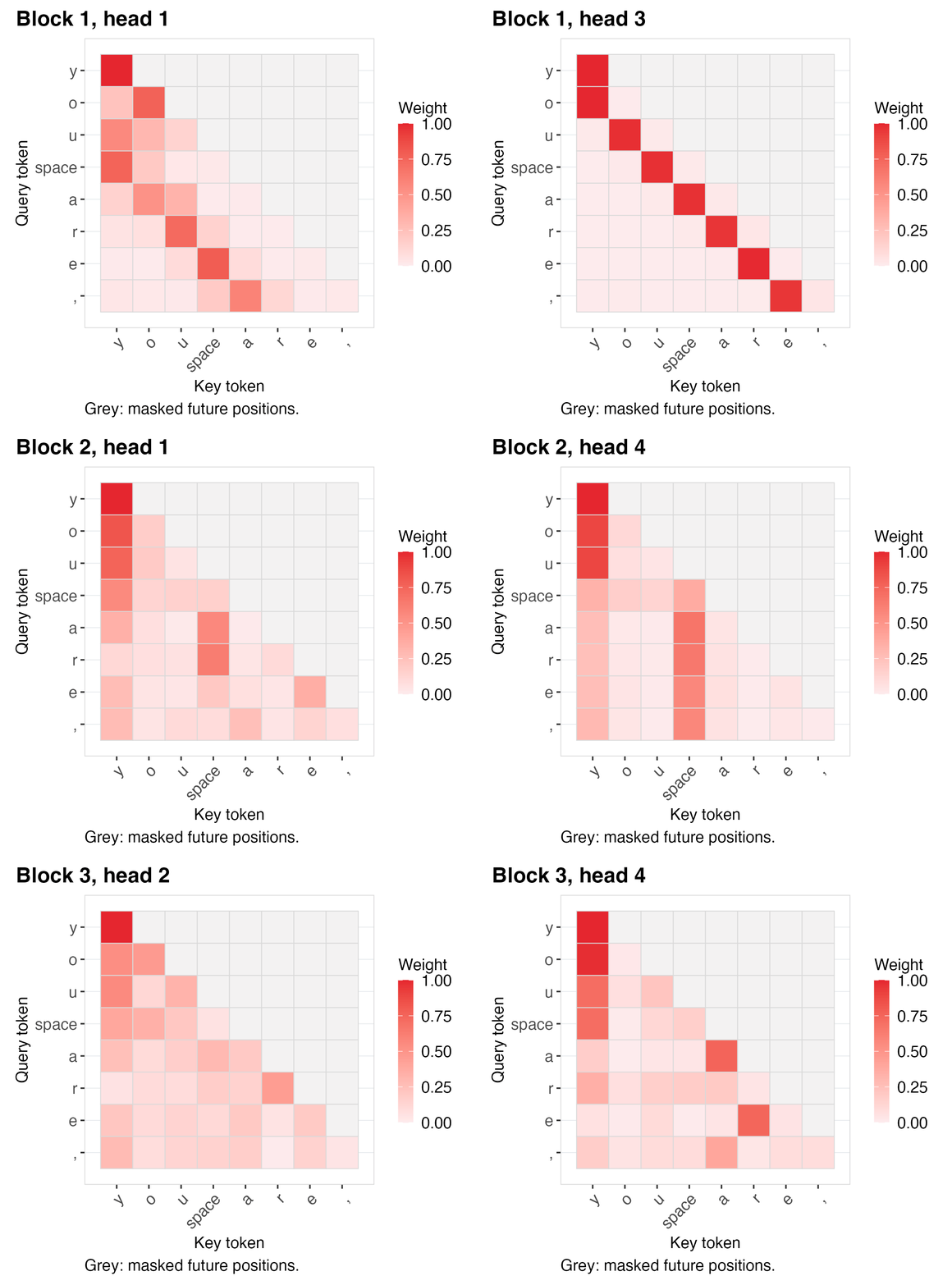
Figure 2. Learned attention across blocks and heads. Each frame shows one attention matrix from the same model and prompt. Rows are query tokens and columns are key tokens. Future positions are causally masked; the remaining weights are normalised independently within each row.

Stacking Transformer blocks

Each block has its own query, key, value, attention-output and feed-forward parameters. Stacking blocks therefore repeats the same computational pattern without reusing the same learned transformation.

The feed-forward sublayer expands each position independently from dimension \(d\) to \(4d\), applies the GELU activation, then projects it back to \(d\). GELU is defined as

where \(\Phi(x)\) is the cumulative distribution function of a standard normal distribution. GPT-2 uses the following tanh approximation,

Here, \(\tanh\) is the hyperbolic tangent. The factor \(\sqrt{2/\pi}\) and fitted coefficient \(0.044715\) make this expression closely approximate the exact normal-distribution form while using elementary operations.

Attention mixes information between sequence positions, while the feed-forward transformation acts independently on the resulting representation at each position. Residual connections preserve the input to both sublayers, and layer normalisation is applied before each transformation.

The attention-output and feed-forward down-projection matrices are initialised with a standard deviation scaled by \(1/\sqrt{2L}\), where \(L\) is the number of Transformer blocks. This follows GPT-2’s residual-path scaling and reduces the growth of residual contributions as depth increases.

How the model predicts the next token

After the final Transformer block, the sequence passes through a final layer normalisation. Each position then contains a \(d\)-dimensional feature vector representing the preceding context available at that position.

GPT-2 shares its input token embeddings with the output projection. We use the same tied embeddings. If \(E\in\mathbb{R}^{V\times d}\) is the token-embedding matrix and \(H\in\mathbb{R}^{T\times d}\) is the final hidden¹ representation, the output logits are

The same matrix that maps token IDs into vectors therefore maps final vectors back to scores over the vocabulary. Weight tying removes a separate \(d\times V\) output matrix and requires gradients from both uses to accumulate into the same parameters.

Softmax converts the logits at each position into a probability distribution over the 256 possible next byte tokens. During generation we use the distribution at the final context position, sample one token, append it to the sequence and repeat.

Learning the parameters

Training minimises next-token cross-entropy over every position in every sampled window. For batch size \(B\) and context length \(T\),

A model assigning equal probability to all 256 byte tokens has loss

nats per token. Training adjusts the parameters so that the observed continuation receives progressively more probability than competing tokens.

The complete backward pass is implemented manually. Gradients pass from cross-entropy through the tied output projection, final layer normalisation, each Transformer block in reverse order, the residual paths, feed-forward layers, multi-head attention and finally the token and position embeddings. The attention backward pass explicitly differentiates the value-weighted output, softmax attention weights, scaled query-key products and the combined QKV projection.

Adam performs the parameter updates with first- and second-moment estimates. The implementation also computes the global gradient norm and clips it when required. Numerical gradient tests compare selected analytical derivatives with finite-difference estimates before longer training runs.

No automatic differentiation system constructs this backward pass. The forward and backward computations use the same R arrays and matrix operations visible in the source code.

Training on Tiny Shakespeare

Tiny Shakespeare contains 1,115,394 characters of dialogue and other text. Because our tokenizer operates on UTF-8 bytes, the model trains on the byte representation of the file rather than a learned word or subword vocabulary.

Our largest experiment uses a context length of 96 tokens, embedding dimension 96, four attention heads, three Transformer blocks and batch size four. It trains for 20,000 parameter updates on the CPU:

Rscript experiments/run.R \
  --input=data/tiny_shakespeare.txt \
  --iterations=20000 \
  --context-length=96 \
  --embedding-size=96 \
  --n-heads=4 \
  --n-layers=3 \
  --batch-size=4 \
  --validation-interval=500 \
  --checkpoint-interval=1000 \
  --plot-detailed

For vocabulary size \(V=256\), context length \(C=96\), embedding dimension \(d=96\) and \(L=3\) blocks, the parameter count is

The tied output projection adds no second vocabulary matrix. The initial and trained checkpoints therefore have the same architecture and exactly the same number of parameters; learning changes their numerical values rather than their size.

Training loss is measured on sampled training windows. Validation uses fixed windows from the held-out validation split and does not update the parameters. The checkpoint with the lowest measured validation loss is saved as the selected model; generated text is not used for model selection. The separate test split remains unused during ordinary checkpoint selection.

In our git repo, each run records its command, resolved settings, corpus checksum, metrics, initial model, best-validation model and resumable latest checkpoint. This keeps the training result associated with the exact data and configuration that produced it. These details were used for the figures shown.

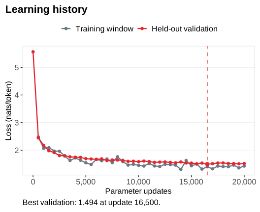
Figure 3. Training and held-out validation loss. Training loss is measured on sampled windows and validation loss on fixed held-out windows. The marked checkpoint is selected by the lowest measured validation loss rather than by the appearance of generated text.

What the model learned

The random and trained models are almost the same size on disk. They contain the same architecture and number of parameters; training changes only the parameter values. The model’s learned behaviour is therefore stored in the particular numerical configuration of those weights. One direct way to inspect that change is to compare their next-token probability distributions for the same prompt.

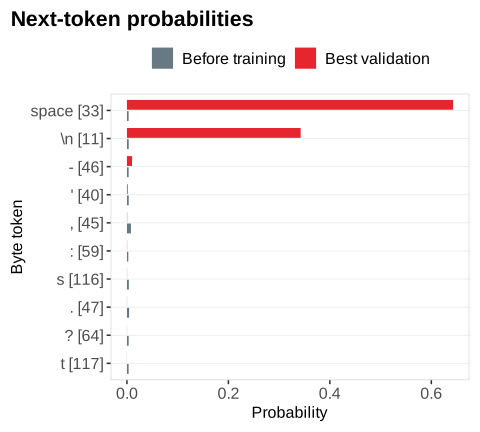
Figure 4. Next-token probabilities before and after training. The figure compares the initial random model with the checkpoint selected by held-out validation, using the same prompt. Training redistributes probability over the byte-token vocabulary according to structure learned from the corpus.

Generation uses the same forward pass but no target token is supplied. The model receives a prompt, predicts a distribution for the next byte, samples one token and appends it to the context. The new sequence is then passed through the model again to predict the following token.

The repository records samples from successive training checkpoints using the same prompt and sampling settings. The generated text becomes progressively more structured as the next-token model improves, although the corpus, context and model remain deliberately small.

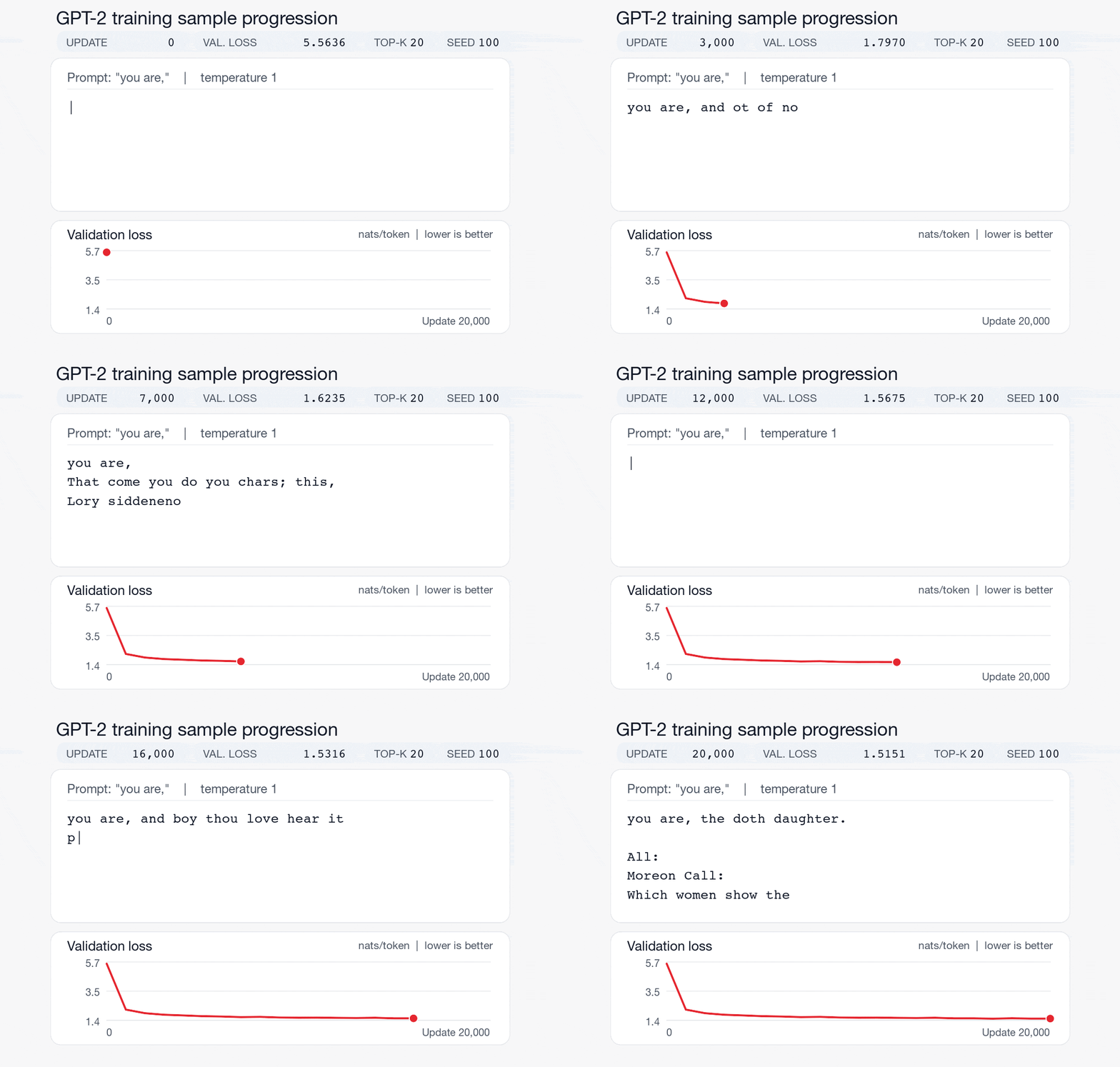
Figure 5. Generated text during training. Each sample uses the same prompt and sampling settings at a different checkpoint. The model begins with random parameters and develops increasingly recognisable local text structure as training proceeds.

What this reproduces and what it does not

Our implementation demo reproduces the main computational structure of a GPT-2-style decoder: learned token and position embeddings, pre-layer normalisation, multi-head masked self-attention, stacked independently parameterised blocks, GELU feed-forward layers, residual connections, a final layer normalisation and tied token embeddings. The loss, backward pass and Adam updates are also implemented directly.

It is not an exact reimplementation of the full OpenAI GPT-2 model. GPT-2 used byte-level BPE rather than raw byte tokens, a much larger vocabulary and context, substantially wider and deeper networks, and a vastly larger training corpus [Radford et al., 2019]. Our model is trained from random parameters on Tiny Shakespeare rather than using OpenAI’s pretrained weights.

Generation is also intentionally simple. The implementation recomputes the active context for every new token rather than caching keys and values from earlier positions. A key-value cache would make inference more efficient without changing the learned attention operation, but would obscure the basic generation path we want to inspect here. The scale is different, but the learning problem is the same.

Our first project exposed this process in a recurrent neural network. The second replaced recurrence with a single-block causal Transformer. This third model adds the depth, multiple attention heads, nonlinear feed-forward transformations and parameter sharing characteristic of GPT-2-style language models while remaining small enough to inspect from input bytes to final gradients.

Applying the same ideas to biological data requires additional structure, including genomic context, dominant and recessive inheritance, and genotype-phenotype relationships. These constraints become part of the model and training design.

For a compact introduction to the broader principles of modern deep learning, we recommend François Fleuret’s The Little Book of Deep Learning. The PDF is freely available, and the pocket-sized physical edition is particularly useful as a concise technical reference.

References

Brown TB, Mann B, Ryder N, et al. Language Models are Few-Shot Learners. Advances in Neural Information Processing Systems. 2020;33:1877-1901.

Fleuret F. The Little Book of Deep Learning. https://fleuret.org/francois/lbdl.html.

OpenAI. Better Language Models and Their Implications. 2019a.

OpenAI. GPT-2: 6-Month Follow-Up. 2019b.

OpenAI. ChatGPT: Optimizing Language Models for Dialogue. 2022.

Radford A, Narasimhan K, Salimans T, Sutskever I. Improving Language Understanding by Generative Pre-Training. OpenAI. 2018.

Radford A, Wu J, Child R, Luan D, Amodei D, Sutskever I. Language Models are Unsupervised Multitask Learners. OpenAI. 2019.

Vaswani A, Shazeer N, Parmar N, et al. Attention Is All You Need. Advances in Neural Information Processing Systems. 2017;30.